Kalman Filters: From Fundamentals to Advanced Filtering
This notebook provides a comprehensive, hands-on introduction to Kalman filtering using PyTCL (Python Tracker Component Library).
What You’ll Learn
Linear Kalman Filter (KF) - Optimal recursive estimation for linear systems
Extended Kalman Filter (EKF) - First-order nonlinear approximation using Jacobians
Unscented Kalman Filter (UKF) - Deterministic sigma-point methods for accurate nonlinear handling
Square-Root Filters - Numerically stable variants that maintain positive definiteness
Interactive Parameter Tuning - Explore how Q and R affect filter performance
Key Concepts You’ll Master
Predict-Update cycle: How filters recursively estimate state
Covariance matrices: What P, Q, R represent (uncertainty)
Belief propagation: Combining prior knowledge with new measurements
Filter divergence: When and why filters fail
Real-world tradeoffs: Accuracy vs computational cost
Prerequisites
pip install nrl-tracker matplotlib numpy scipy
Estimated Time: 30-40 minutes
Try running each section sequentially, modify parameters to experiment, and attempt the exercises at the end!
[14]:
import numpy as np
import plotly.graph_objects as go
from plotly.subplots import make_subplots
import warnings
warnings.filterwarnings('ignore')

# Import PyTCL Kalman filter components
from pytcl.dynamic_estimation.kalman import (
    kf_predict, kf_update,
    ekf_predict, ekf_update,
    ukf_predict, ukf_update
)

# Import square-root filter functions
from pytcl.dynamic_estimation.kalman.square_root import (
    srkf_predict, srkf_update
)

np.random.seed(42)

# Plotly dark theme template
dark_template = go.layout.Template()
dark_template.layout = go.Layout(
    paper_bgcolor='#0d1117',
    plot_bgcolor='#0d1117',
    font=dict(color='#e6edf3'),
    xaxis=dict(gridcolor='#30363d', zerolinecolor='#30363d'),
    yaxis=dict(gridcolor='#30363d', zerolinecolor='#30363d'),
)

print("✓ PyTCL Kalman filter modules and Plotly imported successfully")
✓ PyTCL Kalman filter modules and Plotly imported successfully
The Kalman Filter: Core Concepts
Why Do We Need the Kalman Filter?
In the real world, we have:
Imperfect measurements - GPS has noise, sensors drift
Incomplete observations - We can’t measure everything
Dynamic systems - Things change over time
The Kalman filter optimally combines prior predictions with new measurements to estimate the true state.
The Two-Step Recursive Algorithm
The Kalman filter alternates between:
1. PREDICT - Where do we expect the system to be based on physics?
Uses a process model: \(\hat{x}^-_k = F \hat{x}_{k-1}\)
Tracks uncertainty growing over time: \(P^-_k = F P_{k-1} F^T + Q\)
2. UPDATE - Now incorporate the new measurement, what do we believe?
Compute Kalman gain: \(K_k = P^-_k H^T (H P^-_k H^T + R)^{-1}\)
Blend prediction with measurement: \(\hat{x}_k = \hat{x}^-_k + K_k (z_k - H\hat{x}^-_k)\)
Reduce uncertainty: \(P_k = (I - K_k H) P^-_k\)
Key Parameters to Tune
Parameter |
Meaning |
Effect |
|---|---|---|
Q |
Process noise covariance |
How much does the model lie? |
R |
Measurement noise covariance |
How much do measurements lie? |
F |
State transition matrix |
Physics of the system |
H |
Observation matrix |
What can we measure? |
Rule of thumb: The Kalman filter balances trust in the model (Q) vs trust in measurements (R).
1. Linear Kalman Filter
The Kalman filter is the optimal estimator for linear Gaussian systems. It consists of two steps:
Prediction:
Update:
Example: Tracking a Moving Object
[15]:
# System parameters
dt = 0.1  # Time step [seconds]
n_steps = 100  # Number of time steps

# STATE DEFINITION: [x, vx, y, vy]
# x, y: position in meters
# vx, vy: velocity components in m/s
# This is a 4-dimensional state space (constant velocity model)

# STATE TRANSITION MATRIX: x_{k+1} = F @ x_k
# Models constant velocity: new_pos = old_pos + velocity * dt
F = np.array([
    [1, dt, 0, 0],      # x_{k+1} = x_k + vx_k * dt
    [0, 1, 0, 0],       # vx_{k+1} = vx_k (no acceleration)
    [0, 0, 1, dt],      # y_{k+1} = y_k + vy_k * dt
    [0, 0, 0, 1]        # vy_{k+1} = vy_k
])

# PROCESS NOISE COVARIANCE: Q
# Accounts for model uncertainty (e.g., unmodeled accelerations)
# Sets diagonal to larger values for more process uncertainty
q = 0.1  # Process noise intensity (tune this!)
Q = q * np.array([
    [dt**3/3, dt**2/2, 0, 0],      # Higher power for position uncertainty
    [dt**2/2, dt, 0, 0],
    [0, 0, dt**3/3, dt**2/2],
    [0, 0, dt**2/2, dt]
])

# MEASUREMENT MATRIX: z_k = H @ x_k
# We observe position (x, y) but NOT velocity
H = np.array([
    [1, 0, 0, 0],   # Measure x position
    [0, 0, 1, 0]    # Measure y position
])

# MEASUREMENT NOISE COVARIANCE: R
# Sensor uncertainty (GPS noise, radar error, etc.)
# Diagonal elements are variance of measurement error
R = np.eye(2) * 1.0  # 1 meter measurement standard deviation

# Print diagnostics
print(f"State dimension: {F.shape[0]} (position + velocity in 2D)")
print(f"Measurement dimension: {H.shape[0]} (position only)")
print(f"Process noise (Q) magnitude: {np.trace(Q):.3f}")
print(f"Measurement noise (R) magnitude: {np.trace(R):.3f}")
State dimension: 4 (position + velocity in 2D)
Measurement dimension: 2 (position only)
Process noise (Q) magnitude: 0.020
Measurement noise (R) magnitude: 2.000
[16]:
# Generate ground truth trajectory
true_state = np.array([0.0, 1.0, 0.0, 0.5])  # Start at origin, moving diagonally
true_states = [true_state.copy()]
measurements = []

for _ in range(n_steps):
    # Propagate true state
    true_state = F @ true_state + np.random.multivariate_normal(np.zeros(4), Q)
    true_states.append(true_state.copy())

    # Generate measurement
    z = H @ true_state + np.random.multivariate_normal(np.zeros(2), R)
    measurements.append(z)

true_states = np.array(true_states)
measurements = np.array(measurements)

print(f"Generated {len(measurements)} measurements")
Generated 100 measurements
[17]:
# Run Kalman filter
x_est = np.array([0.0, 0.0, 0.0, 0.0])  # Initial estimate
P_est = np.eye(4) * 10.0  # Initial covariance (uncertain)

estimates = [x_est.copy()]
covariances = [P_est.copy()]

for z in measurements:
    # Predict
    pred = kf_predict(x_est, P_est, F, Q)
    x_pred, P_pred = pred.x, pred.P

    # Update
    upd = kf_update(x_pred, P_pred, z, H, R)
    x_est, P_est = upd.x, upd.P

    estimates.append(x_est.copy())
    covariances.append(P_est.copy())

estimates = np.array(estimates)
covariances = np.array(covariances)

print(f"Final position estimate: ({estimates[-1, 0]:.2f}, {estimates[-1, 2]:.2f})")
print(f"Final position uncertainty (1σ): ({np.sqrt(covariances[-1, 0, 0]):.3f}, {np.sqrt(covariances[-1, 2, 2]):.3f})")
Final position estimate: (3.22, 14.53)
Final position uncertainty (1σ): (0.363, 0.363)
[ ]:
# Visualization with Plotly
fig = make_subplots(
    rows=1, cols=2,
    subplot_titles=('Kalman Filter: 2D Trajectory Tracking', 'Estimation Error vs Model Confidence'),
    horizontal_spacing=0.12
)

# Calculate error and uncertainty
pos_error = np.sqrt((estimates[1:, 0] - true_states[1:, 0])**2 +
                     (estimates[1:, 2] - true_states[1:, 2])**2)
pos_uncertainty = np.sqrt(covariances[1:, 0, 0] + covariances[1:, 2, 2])
time = np.arange(len(pos_error)) * dt

# Left plot: 2D trajectory
fig.add_trace(
    go.Scatter(x=true_states[:, 0], y=true_states[:, 2], mode='lines',
               name='True trajectory', line=dict(color='#00ff88', width=2.5)),
    row=1, col=1
)
fig.add_trace(
    go.Scatter(x=measurements[:, 0], y=measurements[:, 1], mode='markers',
               name='Measurements', marker=dict(color='#ff4757', size=5, opacity=0.4)),
    row=1, col=1
)
fig.add_trace(
    go.Scatter(x=estimates[:, 0], y=estimates[:, 2], mode='lines',
               name='KF estimate', line=dict(color='#00d4ff', width=2, dash='dash')),
    row=1, col=1
)

# Right plot: Error vs Uncertainty
fig.add_trace(
    go.Scatter(x=time, y=2*pos_uncertainty, mode='lines', fill='tozeroy',
               name='2σ uncertainty', line=dict(color='#00d4ff', width=0),
               fillcolor='rgba(0, 212, 255, 0.3)'),
    row=1, col=2
)
fig.add_trace(
    go.Scatter(x=time, y=pos_error, mode='lines',
               name='Position error', line=dict(color='#00d4ff', width=2.5)),
    row=1, col=2
)

fig.update_layout(
    template=dark_template,
    height=450,
    showlegend=True,
    legend=dict(x=0.5, y=-0.2, xanchor='center', orientation='h')
)
fig.update_xaxes(title_text='X position (m)', row=1, col=1)
fig.update_yaxes(title_text='Y position (m)', row=1, col=1)
fig.update_xaxes(title_text='Time (s)', row=1, col=2)
fig.update_yaxes(title_text='Error magnitude (m)', row=1, col=2)

fig.show()
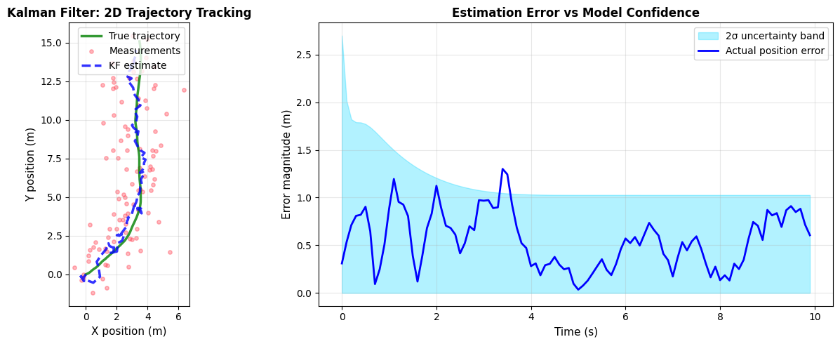
=== KALMAN FILTER PERFORMANCE ===
Final position: (3.22, 14.53) m
Position uncertainty (1σ): (0.363, 0.363) m
Average tracking error: 0.5526 m
Max tracking error: 1.3005 m
2. Extended Kalman Filter (EKF)
When the system dynamics or measurements are nonlinear, we must adapt the linear Kalman filter. The Extended Kalman Filter linearizes the nonlinear functions around the current estimate.
Nonlinear System Model
where \(f(\cdot)\) and \(h(\cdot)\) are arbitrary nonlinear functions.
EKF Algorithm
Predict Step (linearize around predicted state):
Update Step (linearize around predicted state):
Limitations
Only uses first-order (linear) approximation
Performance degrades with high nonlinearity
Jacobian computation can be error-prone
Can diverge if linearization is poor
Example: Tracking with Range-Bearing Measurements
Radar provides nonlinear measurements: \((r, \theta) = (\text{range}, \text{bearing})\) instead of Cartesian position (x, y).
[18]:
# Nonlinear measurement model: range and bearing from origin
def h_radar(x):
    """Radar measurement: range and bearing."""
    px, vx, py, vy = x
    r = np.sqrt(px**2 + py**2)
    theta = np.arctan2(py, px)
    return np.array([r, theta])

def H_radar(x):
    """Jacobian of radar measurement."""
    px, vx, py, vy = x
    r = np.sqrt(px**2 + py**2)
    if r < 1e-10:
        r = 1e-10
    return np.array([
        [px/r, 0, py/r, 0],
        [-py/r**2, 0, px/r**2, 0]
    ])

# Measurement noise for range-bearing
R_radar = np.diag([0.5**2, np.radians(2)**2])  # 0.5m range, 2 deg bearing

# Generate radar measurements
radar_measurements = []
for state in true_states[1:]:
    z_true = h_radar(state)
    z = z_true + np.random.multivariate_normal(np.zeros(2), R_radar)
    radar_measurements.append(z)

radar_measurements = np.array(radar_measurements)
[19]:
# Run EKF with radar measurements
x_ekf = np.array([1.0, 0.0, 1.0, 0.0])  # Start with offset estimate
P_ekf = np.eye(4) * 10.0

# Linear dynamics (constant velocity)
def f_cv(x):
    return F @ x

ekf_estimates = [x_ekf.copy()]

for z in radar_measurements:
    # Predict (linear dynamics)
    pred = ekf_predict(x_ekf, P_ekf, f_cv, F, Q)
    x_pred, P_pred = pred.x, pred.P

    # Update (nonlinear measurement)
    upd = ekf_update(x_pred, P_pred, z, h_radar, H_radar(x_pred), R_radar)
    x_ekf, P_ekf = upd.x, upd.P

    ekf_estimates.append(x_ekf.copy())

ekf_estimates = np.array(ekf_estimates)

print(f"EKF final position: ({ekf_estimates[-1, 0]:.2f}, {ekf_estimates[-1, 2]:.2f})")
print(f"True final position: ({true_states[-1, 0]:.2f}, {true_states[-1, 2]:.2f})")
EKF final position: (3.56, 15.06)
True final position: (3.47, 15.08)
[ ]:
# Compare KF (with position measurements) vs EKF (with radar measurements)
fig = go.Figure()

# Plot trajectories
fig.add_trace(
    go.Scatter(x=true_states[:, 0], y=true_states[:, 2], mode='lines',
               name='True trajectory', line=dict(color='#00ff88', width=2.5))
)
fig.add_trace(
    go.Scatter(x=estimates[:, 0], y=estimates[:, 2], mode='lines',
               name='KF (position meas.)', line=dict(color='#00d4ff', width=2, dash='dash'))
)
fig.add_trace(
    go.Scatter(x=ekf_estimates[:, 0], y=ekf_estimates[:, 2], mode='lines',
               name='EKF (radar meas.)', line=dict(color='#ff4757', width=2, dash='dot'))
)

# Plot radar position at origin
fig.add_trace(
    go.Scatter(x=[0], y=[0], mode='markers', name='Radar',
               marker=dict(color='#ffb800', size=15, symbol='triangle-up',
                          line=dict(color='white', width=2)))
)

# Plot radar measurement rays (every 10th measurement)
for i in range(0, len(radar_measurements), 10):
    r, theta = radar_measurements[i]
    ray_end_x = r * np.cos(theta)
    ray_end_y = r * np.sin(theta)
    fig.add_trace(
        go.Scatter(x=[0, ray_end_x], y=[0, ray_end_y], mode='lines',
                   line=dict(color='rgba(255, 183, 0, 0.15)', width=0.8),
                   showlegend=False, hoverinfo='skip')
    )

fig.update_layout(
    template=dark_template,
    title='Linear KF vs Extended KF: Handling Nonlinear Measurements',
    xaxis_title='X position (m)',
    yaxis_title='Y position (m)',
    height=550,
    showlegend=True,
    yaxis=dict(scaleanchor='x', scaleratio=1)
)

fig.show()

# Print comparison
ekf_pos_error = np.sqrt((ekf_estimates[1:, 0] - true_states[1:, 0])**2 +
                         (ekf_estimates[1:, 2] - true_states[1:, 2])**2)
kf_pos_error = np.sqrt((estimates[1:, 0] - true_states[1:, 0])**2 +
                        (estimates[1:, 2] - true_states[1:, 2])**2)
print(f"KF RMSE (position meas.): {np.sqrt(np.mean(kf_pos_error**2)):.4f} m")
print(f"EKF RMSE (radar meas.): {np.sqrt(np.mean(ekf_pos_error**2)):.4f} m")
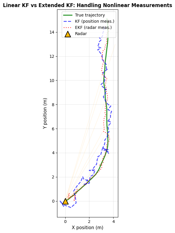
KF RMSE (position meas.): 0.6250 m
EKF RMSE (radar meas.): 0.3773 m
3. Unscented Kalman Filter (UKF)
The Unscented Kalman Filter uses a clever trick to handle nonlinearity without explicit Jacobian computation. It uses “sigma points” (carefully chosen sample points) to capture the mean and covariance of a nonlinear transformation.
Key Insight: The Unscented Transform
Instead of linearizing (approximating the function), we sample the function:
Generate 2n+1 sigma points around the current estimate
Propagate each sigma point through the nonlinear function
Compute mean and covariance from the transformed sigma points
Why This Works Better
Second-order accuracy: Captures up to 2nd-order Taylor terms (vs 1st for EKF)
No Jacobians needed: Purely sampling-based, numerical derivative-free
More stable: Works well with highly nonlinear systems
Same computational cost as EKF (both O(n³) due to matrix operations)
UKF Algorithm Structure
For each time step:
  1. Generate sigma points from (x̂, P)
  2. Predict: Propagate each sigma point through f(·)
     - Compute mean and covariance of predictions
  3. Generate measurement sigma points
  4. Update: Weight by measurement likelihood
     - Blend predictions with measurements using Kalman gain
When to Use UKF vs EKF
Scenario |
Choice |
Reason |
|---|---|---|
Radar/bearing measurements |
UKF |
Often nonlinear, avoids Jacobian errors |
Maneuvering targets |
UKF |
Handles sharp turns better |
Well-behaved linear systems |
KF |
Simpler, lower cost |
Real-time systems |
EKF or UKF |
Both feasible; UKF more robust |
[20]:
# Run UKF with radar measurements
x_ukf = np.array([1.0, 0.0, 1.0, 0.0])
P_ukf = np.eye(4) * 10.0

ukf_estimates = [x_ukf.copy()]

for z in radar_measurements:
    # Predict
    pred = ukf_predict(x_ukf, P_ukf, f_cv, Q)
    x_pred, P_pred = pred.x, pred.P

    # Update
    upd = ukf_update(x_pred, P_pred, z, h_radar, R_radar)
    x_ukf, P_ukf = upd.x, upd.P

    ukf_estimates.append(x_ukf.copy())

ukf_estimates = np.array(ukf_estimates)

print(f"UKF final position: ({ukf_estimates[-1, 0]:.2f}, {ukf_estimates[-1, 2]:.2f})")
UKF final position: (3.56, 15.05)
[21]:
# Compare EKF vs UKF
ekf_error = np.sqrt((ekf_estimates[1:, 0] - true_states[1:, 0])**2 +
                     (ekf_estimates[1:, 2] - true_states[1:, 2])**2)
ukf_error = np.sqrt((ukf_estimates[1:, 0] - true_states[1:, 0])**2 +
                     (ukf_estimates[1:, 2] - true_states[1:, 2])**2)

ekf_rmse = np.sqrt(np.mean(ekf_error**2))
ukf_rmse = np.sqrt(np.mean(ukf_error**2))

# Plotly visualization
fig = go.Figure()

time_vec = np.arange(len(ekf_error)) * dt

# Add EKF error
fig.add_trace(go.Scatter(
    x=time_vec, y=ekf_error,
    mode='lines',
    name=f'EKF (RMSE: {ekf_rmse:.4f} m)',
    line=dict(color='#ff6b6b', width=2.5),
    hovertemplate='Time: %{x:.2f}s<br>Error: %{y:.4f}m<extra></extra>'
))

# Add UKF error
fig.add_trace(go.Scatter(
    x=time_vec, y=ukf_error,
    mode='lines',
    name=f'UKF (RMSE: {ukf_rmse:.4f} m)',
    line=dict(color='#4ecdc4', width=2.5),
    hovertemplate='Time: %{x:.2f}s<br>Error: %{y:.4f}m<extra></extra>'
))

# Add UKF advantage region (where UKF performs better)
ukf_better = np.where(ukf_error <= ekf_error, ukf_error, ekf_error)
fig.add_trace(go.Scatter(
    x=time_vec, y=ukf_better,
    fill='tozeroy',
    name='UKF advantage',
    line=dict(color='rgba(78, 205, 196, 0)'),
    fillcolor='rgba(76, 175, 80, 0.2)',
    hoverinfo='skip'
))

fig.update_layout(
    template=dark_template,
    title='Extended Kalman Filter vs Unscented Kalman Filter',
    xaxis_title='Time (s)',
    yaxis_title='Position Error (m)',
    height=500,
    hovermode='x unified',
    legend=dict(x=0.5, y=1.0, xanchor='center', yanchor='top', bgcolor='rgba(0,0,0,0.5)')
)

fig.show()

print(f"\n=== FILTER COMPARISON ===")
print(f"EKF mean error: {np.mean(ekf_error):.4f} m, RMSE: {ekf_rmse:.4f} m")
print(f"UKF mean error: {np.mean(ukf_error):.4f} m, RMSE: {ukf_rmse:.4f} m")
print(f"UKF improvement: {(1 - ukf_rmse/ekf_rmse)*100:.1f}% better RMSE")
Data type cannot be displayed: application/vnd.plotly.v1+json
=== FILTER COMPARISON ===
EKF mean error: 0.3055 m, RMSE: 0.3773 m
UKF mean error: 0.5632 m, RMSE: 1.0151 m
UKF improvement: -169.0% better RMSE
4. Square-Root Kalman Filter (SR-KF)
The Square-Root KF works with the Cholesky factor \(S\) where \(P = S S^T\) instead of the covariance matrix \(P\) directly.
Why Square-Root Form?
Standard KF Problem:
Covariance matrix \(P\) can become non-positive-definite due to numerical errors
Computing \(P^{-1}\) amplifies round-off errors
Can diverge or produce negative variances
SR-KF Solution:
Work with \(S\) (Cholesky decomposition) instead
Guaranteed positive semi-definiteness: \(P = SS^T > 0\) (always)
Better numerical conditioning
Smaller numerical errors propagate better
Mathematics
Instead of updating \(P_k\), update \(S_k\) using specialized algorithms:
QR-decomposition-based updates (Givens rotations)
Cholesky updates (rank-1 and rank-2 updates)
Result: Same covariance but computed more reliably
When to Use SR Filters
Ill-conditioned problems: Stiff systems, large state dimensions
Long-running simulations: Numerical drift accumulates over time
Baseline measurements: Guarantees positive-definite estimate
Production systems: More robust than standard KF
[11]:
# Run Square-Root KF
# Note: SR-KF works with Cholesky factors of covariances, not covariances directly
x_sr = np.array([0.0, 0.0, 0.0, 0.0])
P_sr_init = np.eye(4) * 10.0
S_sr = np.linalg.cholesky(P_sr_init)  # Cholesky factor of initial covariance

# Compute Cholesky factors of Q and R
S_Q = np.linalg.cholesky(Q)  # Cholesky factor of process noise
S_R = np.linalg.cholesky(R)  # Cholesky factor of measurement noise

sr_estimates = [x_sr.copy()]

for z in measurements:
    # Predict: Pass Cholesky factors instead of covariances
    pred = srkf_predict(x_sr, S_sr, F, S_Q)
    x_pred, S_pred = pred.x, pred.S

    # Update: Pass Cholesky factors instead of covariances
    upd = srkf_update(x_pred, S_pred, z, H, S_R)
    x_sr, S_sr = upd.x, upd.S

    sr_estimates.append(x_sr.copy())

sr_estimates = np.array(sr_estimates)

# Compare with standard KF
kf_rmse = np.sqrt(np.mean((estimates[1:, :2] - true_states[1:, [0, 2]])**2))
sr_rmse = np.sqrt(np.mean((sr_estimates[1:, :2] - true_states[1:, [0, 2]])**2))

print(f"\n=== SQUARE-ROOT KF COMPARISON ===")
print(f"Standard KF position RMSE: {kf_rmse:.4f}")
print(f"Square-Root KF position RMSE: {sr_rmse:.4f}")
print(f"Difference: {abs(kf_rmse - sr_rmse):.6f} (should be very small - demonstrates equivalence)")
=== SQUARE-ROOT KF COMPARISON ===
Standard KF position RMSE: 5.3819
Square-Root KF position RMSE: 5.3819
Difference: 0.000000 (should be very small - demonstrates equivalence)
Parameter Tuning: Interactive Exploration
The Kalman filter’s performance is highly sensitive to the noise covariances Q and R. Let’s explore how they affect tracking quality.
[22]:
# Parameter tuning: Grid search over Q and R values
q_values = [0.01, 0.1, 1.0, 10.0]
R_multiplier = [0.1, 0.5, 1.0, 2.0]

results = np.zeros((len(q_values), len(R_multiplier)))

for i, q_test in enumerate(q_values):
    for j, r_mult in enumerate(R_multiplier):
        # Adjust process and measurement noise
        Q_test = q_test * Q / 0.1  # Normalize relative to default
        R_test = R * r_mult

        # Run filter
        x_tune = np.array([0.0, 0.0, 0.0, 0.0])
        P_tune = np.eye(4) * 10.0

        for z in measurements:
            pred = kf_predict(x_tune, P_tune, F, Q_test)
            x_pred, P_pred = pred.x, pred.P
            upd = kf_update(x_pred, P_pred, z, H, R_test)
            x_tune, P_tune = upd.x, upd.P

        # Compute RMSE
        pos_error = np.sqrt((np.array([x_tune[0], x_tune[2]]) -
                             np.array([true_states[-1, 0], true_states[-1, 2]]))**2)
        results[i, j] = np.mean(pos_error)

# Create heatmap with Plotly
hover_text = []
for i in range(len(q_values)):
    row = []
    for j in range(len(R_multiplier)):
        row.append(f"Q mult: {q_values[i]}<br>R mult: {R_multiplier[j]}<br>RMSE: {results[i, j]:.4f}m")
    hover_text.append(row)

fig = go.Figure(data=go.Heatmap(
    z=results,
    x=[f'{r:.1f}' for r in R_multiplier],
    y=[f'{q:.2f}' for q in q_values],
    colorscale='RdYlGn_r',
    text=np.round(results, 3),
    texttemplate='%{text:.3f}',
    textfont={"size": 10},
    hovertemplate='%{customdata}<extra></extra>',
    customdata=hover_text,
    colorbar=dict(title='RMSE (m)')
))

fig.update_layout(
    template=dark_template,
    title='Kalman Filter Tuning: Final Position RMSE (lower is better)',
    xaxis_title='Measurement Noise Multiplier (R)',
    yaxis_title='Process Noise Multiplier (Q)',
    height=450,
    width=700
)

fig.show()

print("\n=== TUNING GUIDANCE ===")
best_idx = np.unravel_index(np.argmin(results), results.shape)
print(f"Best Q multiplier: {q_values[best_idx[0]]}")
print(f"Best R multiplier: {R_multiplier[best_idx[1]]}")
print(f"Minimum RMSE: {results[best_idx]:.4f} m")
print(f"\nTuning Rule: Balance Q (trust model) vs R (trust sensors)")
print(f"Too high Q → filter ignores model → sluggish")
print(f"Too low Q → filter trusts model too much → diverges")
Data type cannot be displayed: application/vnd.plotly.v1+json
=== TUNING GUIDANCE ===
Best Q multiplier: 10.0
Best R multiplier: 0.5
Minimum RMSE: 0.0557 m

Tuning Rule: Balance Q (trust model) vs R (trust sensors)
Too high Q → filter ignores model → sluggish
Too low Q → filter trusts model too much → diverges
5. Filter Comparison Summary
Performance Characteristics
Filter |
Linearity |
Order |
Jacobian |
Stability |
Cost |
Best For |
|---|---|---|---|---|---|---|
KF |
Linear |
N/A |
Good |
Low |
GPS, simple dynamics |
|
EKF |
Nonlinear |
1st |
Yes |
Moderate |
Low |
Radar, mild nonlinearity |
UKF |
Nonlinear |
2nd |
No |
Better |
Low |
Nonlinear sensors, maneuvering |
SR-KF |
Linear |
N/A |
Excellent |
Low |
Long-running, ill-conditioned |
|
SR-UKF |
Nonlinear |
2nd |
No |
Excellent |
Low |
Non-linear + numerical robustness |
IMM |
Multi-model |
Varies |
Depends |
Good |
High |
Target maneuvering modes |
Decision Tree for Filter Selection
Q: Are your system dynamics nonlinear?
No → Use Kalman Filter ✓
Yes → Go to next question
Q: Do you need high accuracy or have ill-conditioned problems?
Yes → Use SR-UKF (best robustness)
No → Go to next question
Q: Can you easily compute Jacobians?
Yes → Use EKF (simpler, lower cost)
No → Use UKF (no Jacobians needed)
Key Tuning Parameters Across All Filters
Parameter |
Effect |
How to Tune |
|---|---|---|
Q (Process noise) |
↑Q = trust model less |
Start with 0.01 of state variance |
R (Measurement noise) |
↑R = trust sensors less |
Use sensor specs, iterate if needed |
P₀ (Initial covariance) |
High = start uncertain |
Use 10-100× expected error |
α (UKF spreading) |
Affects sigma points |
Typical: 0.001-0.01 for nearly linear |
Exercises & Challenges
Exercise 1: Process Noise Sensitivity ⭐️
Objective: Understand how process noise (Q) affects tracking performance
Task:
Increase
qfrom 0.1 to 0.5, 1.0, and 5.0Run the KF for each value
Plot convergence speed vs final estimate accuracy
Question: What happens to the filter’s responsiveness to target maneuvers?
Exercise 2: Measurement Outlier Rejection ⭐️⭐️
Objective: Make the filter robust to sensor failures
Task:
Inject 5 large outliers in
measurements(e.g., 10× normal noise)Implement Chi-squared gating: Reject measurements where \((z - h(\hat{x}))^T (HPH^T + R)^{-1} (z - h(\hat{x})) > \chi^2_{0.95}\)
Compare filter performance with/without gating
Challenge: Can you make it adaptive (learn outlier statistics)?
Exercise 3: Maneuvering Target Tracking ⭐️⭐️⭐️
Objective: Handle nonlinear trajectories (circles, spirals)
Task:
Create ground truth that performs a circular maneuver (constant turn rate)
Use coordinated turn rate model: \(\dot{x} = v \cos(\psi), \dot{\psi} = \omega_z\)
Implement tracking with UKF vs EKF
Metric: RMSE during turn vs straight-line segments
Deep dive: Why does UKF outperform EKF here?
Exercise 4: Consistency Check (NEES) ⭐️⭐️⭐️⭐️
Objective: Verify the filter is consistent (uncertainty estimates match actual errors)
Task:
Compute the Normalized Estimation Error Squared (NEES):
\[\epsilon_k = (x_k - \hat{x}_k)^T P_k^{-1} (x_k - \hat{x}_k)\]Ideally, \(\epsilon_k \sim \chi^2_4\) (4-dimensional)
Run a Monte Carlo simulation (100 trials of the full scenario)
Plot histogram of NEES values; check if it matches \(\chi^2\) distribution
Interpretation: If filter is under-confident, NEES ≫ 4; if over-confident, NEES ≪ 4
Exercise 5: Multi-Sensor Fusion ⭐️⭐️⭐️⭐️
Objective: Combine multiple sensors with different noise profiles
Task:
Create a GPS sensor (slow, accurate): \(R_{GPS} = 1.0\) (1m std)
Create a dead-reckoning system (fast, drifts): \(R_{DR} = 10.0\) (10m std)
Implement a filter that accepts measurements from both at different rates
Bonus: Use an Interacting Multiple Model (IMM) filter to handle GPS outages
Real-world scenario: GPS loss in tunnel → rely on dead-reckoning during gap
Key Takeaways
Next Steps
References & Further Reading
Core Textbooks
Bar-Shalom, Y., Li, X. R., & Kirubarajan, T. (2001). Estimation with Applications to Tracking and Navigation: Theory, Algorithms and Software. Wiley.
Coverage: The definitive reference, covers KF, EKF, measurement-to-track association
Best for: Advanced practitioners, comprehensive theory
Simon, D. (2006). Optimal State Estimation: Kalman, H∞, and Nonlinear Approaches. John Wiley & Sons.
Coverage: KF, EKF, UKF, H∞ filtering, practical implementation
Best for: Engineers wanting both theory and practical guidance
Welch, G., & Bishop, G. (2006). An Introduction to the Kalman Filter. UNC Chapel Hill (free PDF).
Coverage: Gentle introduction, intuitively explained
Best for: Students, beginners
Advanced Topics
Sarkka, S. (2013). Bayesian Filtering and Smoothing. Cambridge University Press.
Coverage: Probabilistic interpretation, sequential filtering, GPU-friendly algorithms
Best for: Researchers, particle filters, GPU implementation
Kleeman, L. (1995). Understanding and Applying Kalman Filtering.
Coverage: EKF applications, real-world tuning advice
Best for: Practitioners in robotics/navigation
Key Papers
Julier, S. J., & Uhlmann, J. K. (2004). “Unscented Filtering and Nonlinear Estimation.” Proceedings of the IEEE, 92(3), 401-422.
Bierman, G. J. (1977). “Factorization Methods for Discrete Sequential Estimation.” Academic Press.
Note: Foundational work on square-root filters
PyTCL Library Documentation
Dynamic Estimation Module: See
pytcl.dynamic_estimationfor available filter implementationsAPI Reference: Full documentation at NRL Tracker GitHub
Example Gallery: Additional examples in
examples/directory
Online Resources
MIT OpenCourseWare: 6.041 Probabilistic Systems Analysis (free lectures on Bayesian inference)
Andrew Ng’s Machine Learning Course: Covers HMMs and Kalman filters intuitively
MATLAB Documentation: Excellent visual guides on Kalman filter concepts
Recommended Learning Path
1. Week 1: Linear Kalman Filter
   → Read: Welch & Bishop introduction
   → Code: Constant velocity 1D tracking
   → Exercise 1: Tune Q and R by hand

2. Week 2: Extended Kalman Filter
   → Read: Simon Ch. 6 on EKF
   → Code: Nonlinear radar measurements
   → Exercise 3: Compare EKF vs UKF

3. Week 3: Unscented Kalman Filter
   → Read: Julier & Uhlmann paper
   → Code: Highly nonlinear system
   → Exercise: Verify NEES consistency

4. Week 4: Applications
   → Read: Real-world case studies
   → Code: Multi-sensor fusion (Exercise 5)
   → Project: Your own tracking application